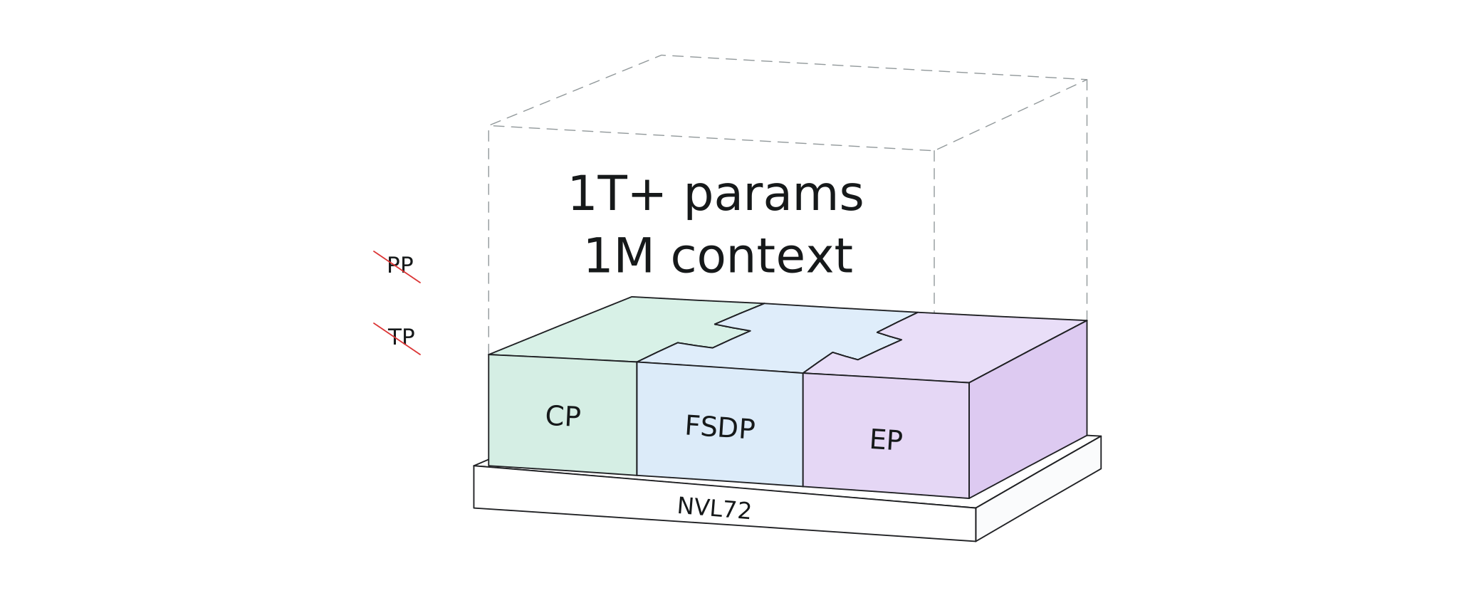
In the previous post I complained at length about pipeline parallelism. This post pays off that debt: without PP, where do the parameters go, how do we split long contexts, and what about cross-node communication?

Before getting into it, let’s make some assumptions and set some constraints to shrink the design space. Otherwise, if we keep bolting on every feature, we end up with another Megatron, and at that point we might as well just use Megatron.

Constraints

Support trillion-scale parameter counts (1T+ params)
Support one-million-token context length
NVL72 cluster
No reliance on CPU offload for model state or activations.

Deriving the Scheme

Let’s start with a rough count of how many GPUs we need just to have enough memory. First, the resident memory per parameter:

FP32 master weights: 4 B
FP32 AdamW optimizer state: 4+4 B
FP32 gradients: 4 B
BF16 weights: 2 B
Note: Muon would shrink the optimizer state, but to be conservative we take 8 B for optimizer state here.
Note: BF16 weights can be rebuilt from the master weights, so in theory they don’t have to stay resident in memory, but most implementations keep them there. To be conservative, we count them as resident.
Note: also to be conservative, we don’t consider low-precision quantization here.

At a trillion parameters, that’s 18 TB of memory. Under this precision and state layout, sharding changes where the state lives, not the deduplicated total. A GB200 has 200 GB of memory, so resident state alone needs at least 90 GPUs. In other words, it doesn’t fit in one NVLink domain, and some communication has to go over RDMA.

So let’s first solve parameter sharding.

Since we’re considering trillion-parameter models, and every model at this scale today is MoE with experts making up over 98% of the parameters, solving expert sharding basically solves the resident memory problem.

Thanks to the NVL72 interconnect, we can directly use EP=64 for communication and compute, and EP dispatch/combine stays inside NVLink without touching RDMA. A pure-NVLink kernel like this is much easier to implement. The DeepEP and DualPipe that DeepSeek-V3 racked its brains over for cross-node communication are no longer needed. (Once again, DeepEP really is exquisite; more of that story in an earlier post.)

But obviously EP=64 alone still can’t hold all the parameters. So we take another cut at the expert parameters with FSDP, say adding a dimension eFSDP=4. That gives 256 GPUs in total. One expert’s parameters are split across 4 GPUs in 4 racks. While computing the current layer, FSDP prefetches the next layer’s parameters. After the FSDP all-gather, every rack has the full parameters for the current layer. This guarantees the EP=64 communication still happens inside NVLink.

OK, with the 98% expert parameters handled, the remaining 2% dense parameters can be dealt with however we like; just shard them with FSDP.

With parameter placement solved, let’s compute the dynamic memory usage. Take the GLM-5.2 architecture as an example:

Assume we recompute every layer during the backward pass; we still need to save at least each layer’s activations. 78 layers * 6144 hidden * BF16 = 0.958 MB/token
We also save the DSA Indexer’s top-k results, since that part runs relatively slowly. 21 layers * top 2048 * int32 = 0.172 MB/token
EP communication buffers. Each token needs 6144 BF16 hidden + FP32 probs * 256 experts = 13312 B. Consider the worst case where every EP rank sends to the current rank, i.e., amplified by EP times. 13312 B * 64 = 0.852 MB/token
Per-layer recompute plus backward needs roughly 2.5 MB/token.
FSDP: 753B params / 78 layers * (2% dense params + 98% expert params / EP 64) * (BF16 current-layer weights + BF16 prefetched next-layer weights + FP32 gradient buffer) = 2.727 GB.

Again thanks to the NVL72 interconnect, we can directly turn on CP=64 and split one sequence across a whole rack. Dynamic memory per GPU is 1048576 * (0.958 + 0.172 + 0.852 + 2.5) / 64 = 73.433 GB. Add the parameter memory 753 * 18 * (2% / 64 + 98% / 256) = 56.122 GB and the FSDP 2.727 GB, for about 133 GB total. That leaves 67 GB of headroom under 200 GB for other temporary buffers we haven’t modeled.

If FA4 PR 2816 gets merged, forward and backward each save about another 0.5 MB/token. Then it fits even when shrunk to 128 GPUs. Or, staying at 256 GPUs, the microbatch can go from 1 to 2.

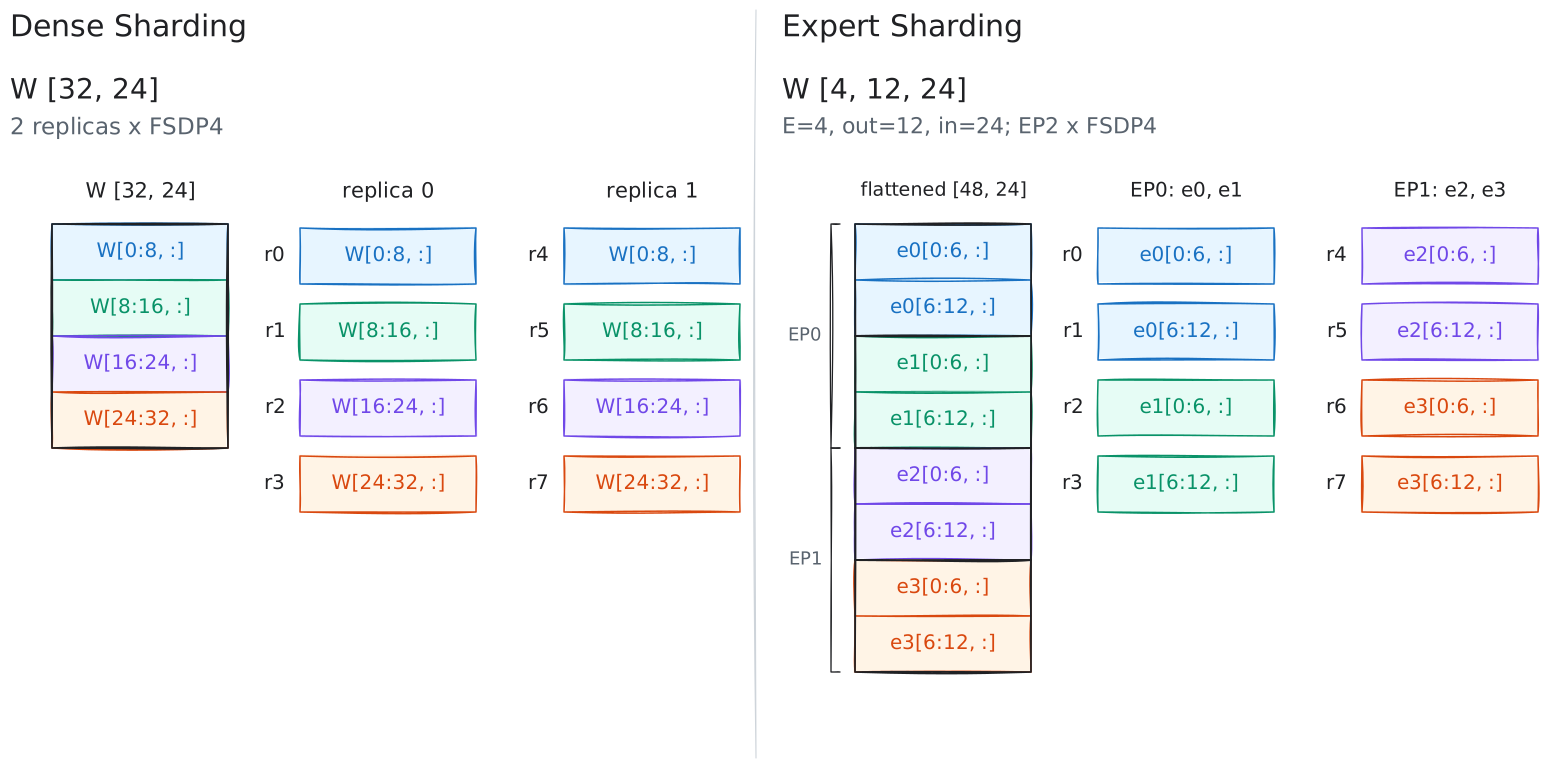
At this point the skeleton of the whole scheme is already out: three forms of parallelism, FSDP x CP x EP. Expert parameters and dense parameters use different sharding:

Dense mesh: (d_rep, fsdp, cp)
Expert mesh: (e_fsdp, ep)
ep <= NVL and fsdp * cp <= NVL, so that all critical-path communication that happens once per layer stays inside NVLink.
d_rep * fsdp * cp == e_fsdp * ep == world
Dense parameters are sharded within fsdp x cp and replicated across d_rep.
Expert parameters are spread across ep, and each rank further shards along e_fsdp.
The size of cp is independent of ep; it depends on the context length to support and the memory footprint.
Total data parallelism (DP) is d_rep * fsdp.
To scale to tens of thousands of GPUs, add an e_rep dimension.

The 256-GPU 1M-context example above uses

(d_rep, fsdp, cp) = (4, 1, 64)
(e_fsdp, ep) = (4, 64)

Hiding eFSDP Communication

The derivation above settles the memory concerns; now let’s analyze communication. The biggest worry is whether FSDP communication can be hidden behind each layer’s compute. We keep using the GLM-5.2 architecture for the numbers.

First estimate the size of one layer’s expert parameters that each rank needs to hold in full: 753B params / 78 layers * 98% expert params * BF16 / EP 64 ≈ 300 MB
These parameters are split into e_fsdp shards, so each rank needs to receive a fraction (e_fsdp - 1) / e_fsdp. When e_fsdp is large, this fraction approaches 1. We take the upper bound as the worst case. So in each layer’s forward pass, the FSDP all-gather needs to receive 300 MB.
The weight shards are freed after the forward pass, so the backward pass needs another 300 MB FSDP all-gather. Then the FP32 gradients need a 600 MB FSDP reduce-scatter.
So the total communication per layer is about 1200 MB.
Each GB200 typically comes with 400 Gbps of RDMA bandwidth; GB300 has 800 Gbps. We use 45 GB/s for the estimate.
So the eFSDP communication time per layer is about 27 ms.

Notice that this communication volume is independent of the number of input tokens. So we can rephrase “can eFSDP communication be hidden” as “how many tokens does a microbatch need at minimum so there is enough compute to hide eFSDP communication”.

Now let’s estimate the compute.

First, the number of active parameters per layer: 753B params / 78 layers * (2% dense params + 98% expert params * 8/256) ≈ 0.5B.
Consider the linear layers first. The forward pass needs 2 FLOP/param/token; in the backward pass, recompute, dgrad, and wgrad each need 2 FLOP/param/token. So the total is 4 GFLOP/token.
Attention compute is messy to model, so instead of modeling it carefully we simply assume a time ratio between attention and the linear layers. From profile data, it’s 2:1 at 256k context (262,144 tokens) and 4:1 at 1M context. We conservatively use 2:1 here (underestimating attention compute time at 1M context).
GB200’s paper spec is 2.5 PFLOP/s; assume 80% of theoretical is achievable (an overestimate).
Conservatively (overestimating communication time, underestimating compute time), the number of tokens needed to hide eFSDP communication is (2.5 PFLOP/s * 80%) * 27 ms / (4 GFLOP * (1 + 2)) ≈ 4,500

That is, a microbatch only needs 5000 tokens per GPU to cover the eFSDP communication. Easy.

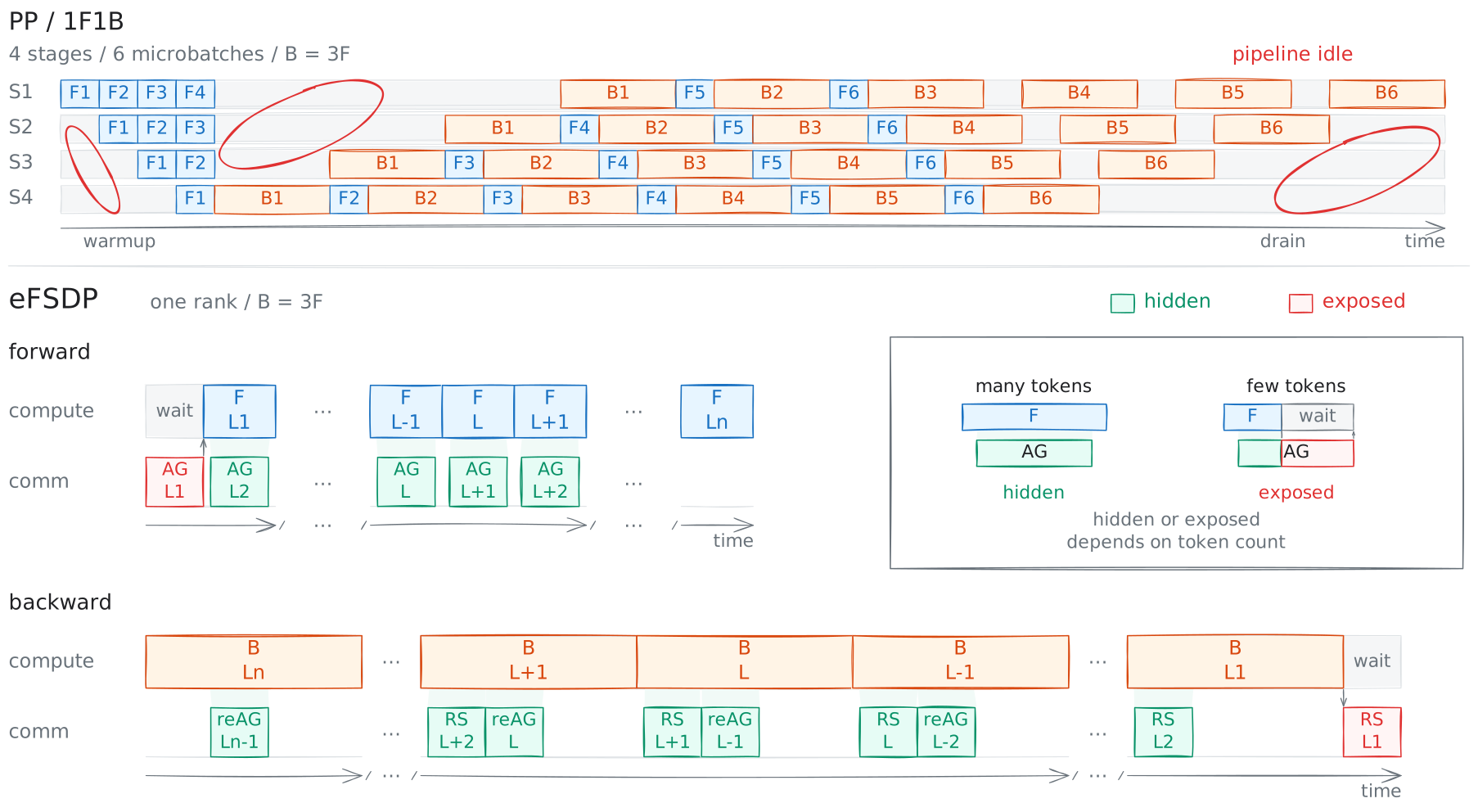
This analysis also explains a big difference between eFSDP and PP. PP’s waste in communication and compute is structural. You can only reduce the bubble by tuning the number of stages and microbatches, or, like Zero Bubble, eliminate it in theory with a more complex schedule and more memory. eFSDP, on the other hand, is a comparison of compute and communication in time: once the input length exceeds the threshold, the extra cost of communication is nearly zero.

Of course eFSDP has structural waste too. The all-gather of the first layer’s forward pass and the reduce-scatter of the last layer’s backward pass cannot be hidden. But a 1/78 cost is relatively easy to accept, given that getting PP’s bubble down to 1.28% is no easy feat.

CP

River God: Young woodcutter, is the axe you dropped this golden one, this silver one, or this iron one?

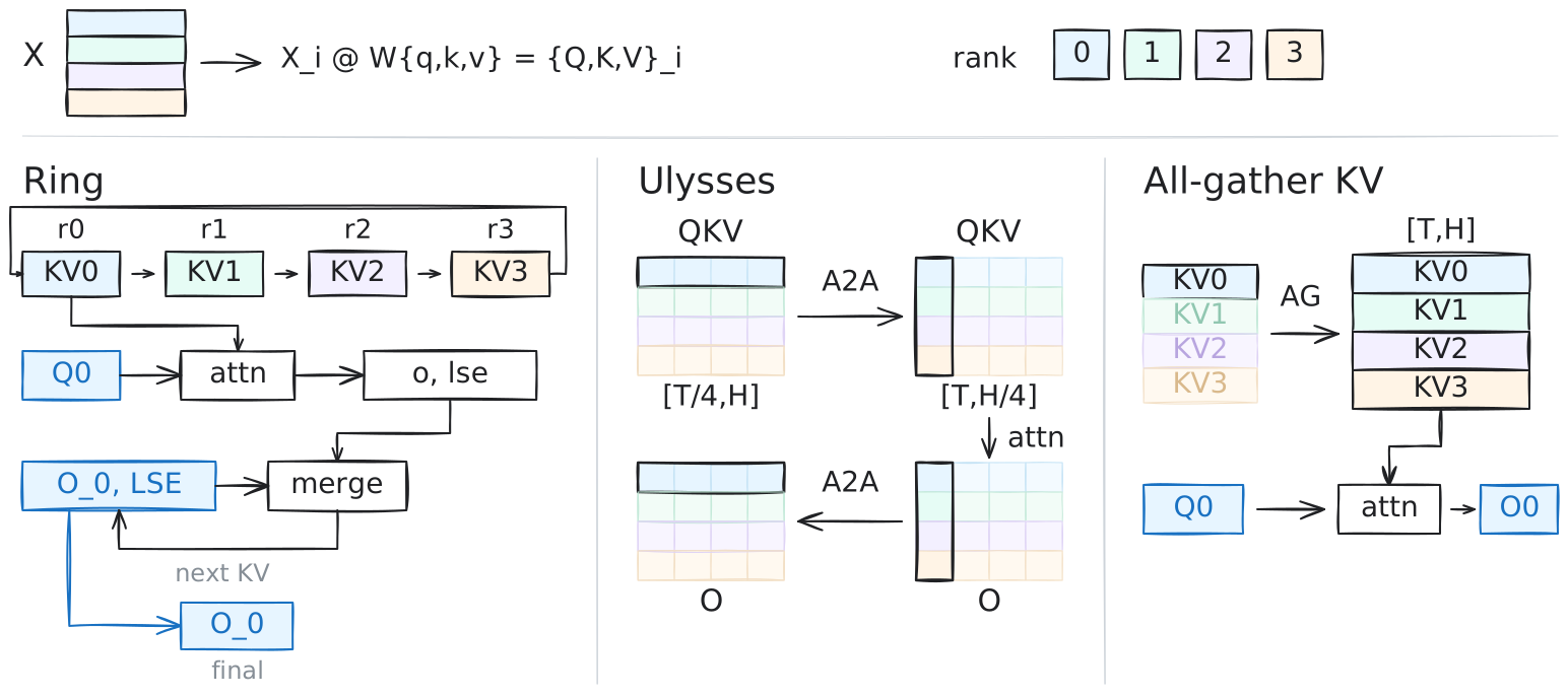
Context Parallelism (CP) cuts along the sequence dimension, so one full sequence is computed across multiple GPUs. Most of the computation operates on a single token’s hidden state and has no notion of a sequence, so CP doesn’t affect it. Only attention crosses tokens and has to deal with the sequence. There are several CP schemes:

Ring Attention: Q stays local, KV blocks are passed around a ring, and LSE is merged as you compute. Communication is point-to-point, so it’s sometimes called P2P CP. The cost is multiple rounds of communication, state merging, reduced kernel efficiency, and possibly needing to modify the attention kernel’s implementation.
Ulysses: Use all-to-all to transpose the original sequence-dimension split into a split by attention heads, run a normal attention kernel, then all-to-all back. Hence sometimes called A2A CP. The upside is no kernel changes and no LSE merging. The downside is being limited by the number of attention heads, and Q/K/V/O all need communication.
USP: Combine the two above, Ring over RDMA and Ulysses over NVLink. A bit too complex, and not needed under NVL72 anyway.
All-gather KV: As the name says, all-gather the KV first, then local Q can compute normally against the global KV. The upside is that it’s extremely simple to implement, with no limit on the number of attention heads and no constraint on the kernel implementation. The downside is that the global KV has to be transferred once, and there has to be memory to temporarily hold this layer’s global KV.

Modern architectures (GQA, MLA, DSA) all aggressively compress the KV size, so all-gather KV comes out both easy to write and fast. MLA transfers the latent KV. DSA needs to transfer the Indexer’s K in addition to the latent KV.

Linear attention (GDN, KDA) has a recurrent state, so unlike ordinary softmax attention, it can’t use the all-gather KV scheme. Besides the two options of recompute and Ulysses, there is also the ingenious KCP. I haven’t figured KCP out yet, but it sure runs fast.

Also worth mentioning: the causal mask makes the compute uneven across CP ranks, with later ranks needing more compute, which is especially pronounced at long context. A zig-zag arrangement can be added to fix the load imbalance.

TP

This minimalist parallelism scheme keeps only FSDP x CP x EP. Not only did we cut PP, we also didn’t add TP. TP actually wouldn’t add much implementation or maintenance burden. It’s left out mainly to stay minimal, and because TP can’t guarantee much extra benefit.

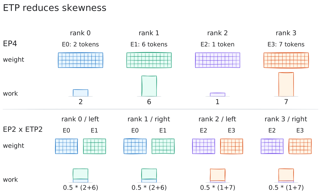
Let’s first discuss tensor parallelism for experts, also called ETP. ETP and EP can be used together: split experts by rows or columns into ETP shards, then do EP as usual, with the compute dimension shrunk by ETP times, and after computing, do TP communication and aggregation.

ETP and EP partition the NVLink domain orthogonally, so if you set ETP=4, the other side can only drop to EP=16. What’s the benefit of doing this?

Let \(A_i\) be the load on each GPU under EP=64, and \(B_g\) the load per group under ETP=4 EP=16. Then

\[B_g = \frac{A_{4g} + A_{4g+1} + A_{4g+2} + A_{4g+3}}{4}\]

Essentially, each GPU’s load is replaced by the average load of 4 GPUs. Define load skew as

\[\operatorname{skew}(X) \coloneqq \frac{\max_{j} X_j}{\overline{X}}\]

Total compute and average load are unchanged, and an average never exceeds the maximum within its group, so adding ETP lowers the load skew:

\[\overline{B} = \overline{A}, \quad \max_{g} B_g \le \max_{i} A_i \; \Longrightarrow \operatorname{skew}(B) \le \operatorname{skew}(A)\]

So what’s the price?

GEMMs get slower. Note that the expert intermediate dimension is already small (2048 or even 1536), and after the ETP cut it gets even smaller.
More EP communication. A token has to reach all 4 GPUs of an ETP group, so EP communication volume becomes 4x that of no ETP.
More activation memory, for the same reason as above.
Each layer gains a reduce-scatter and an all-reduce inside the ETP group, adding two more synchronization points.

So better load skew does not mean the whole thing runs faster.

And if the goal is just to fix load imbalance, there are other approaches. For example, MoonEP recently achieved perfect balance through dynamic redundant experts and online planning.

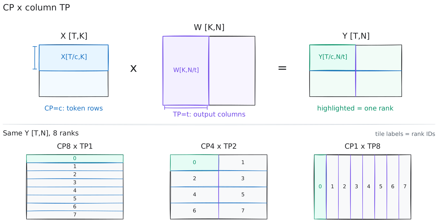
On the other side, consider TP for the dense projections and the attention mechanism.

For dense projections, we already split along the token dimension with CP, so their compute is already parallelized. On top of that, in theory we could still add TP to further split inside the matrix multiplication. But note that CP and TP partition the NVLink domain orthogonally: adding TP means lowering CP, so their contributions to parallelizing the dense projections are in conflict.

Attention has to be discussed case by case.

GQA: Qwen3.5 has only 2 KV heads, so TP greater than 2 requires replicating KV. Conversely, for CP, few KV heads make all-gather KV very cheap.
MLA: After expanding into MHA there are plenty of heads, so no problem there. But in RL post-training, to reduce numerical discrepancy between the training framework and the inference engine, one may want to compute in the matrix-absorbed form. For that case, it seems none of the current kernels support TP.
DSA: The current kernel implementations basically pad the number of heads to a multiple of 64 internally, which limits the speedup TP can bring.
GDN: The kernels seem to support it, but GDN doesn’t have many heads either, so the speedup may be limited.

Overall, TP and CP compete for the same parallelism ceiling, and TP usually comes with lower kernel efficiency, so without measuring, it’s hard to say how much faster it would actually be. CP is far easier to implement than TP and scales very conveniently to 64 GPUs. So for simplicity, I chose only CP here and dropped TP.

Bonus: What If There’s No NVL72?

We assumed an NVL72 cluster above. But if all you can rent is an NVL8 cluster, does this scheme still apply? Here we consider B300 rather than B200, first because B300 has much more memory at 309 GB, and second because B300 comes with 800 Gbps of RDMA.

Let’s relax the context length first and consider 256k context (262,144 tokens per sequence). Carrying over the earlier calculations:

(e_fsdp, ep) = (32, 8), cp=8, d_rep * fsdp == 32
Each CP group’s microbatch holds one 256k sequence, so the number of tokens per GPU is at least 262144 * 32 / 256 = 32768.
Dynamic memory
- EP communication buffers shrink: 13312 B * 8 = 0.106 MB/token
- Other dynamic memory stays the same: activation checkpoints 0.958 MB/token, DSA Indexer top-k 0.172 MB/token, per-layer recompute plus backward 1.5 MB/token (assuming FA4 PR 2816 is merged)
- FSDP: 753B params / 78 layers * (2% dense params + 98% expert params / EP 8) * (BF16 current-layer weights + BF16 prefetched next-layer weights + FP32 gradient buffer) = 11.005 GB
- Total dynamic memory is 32768 * (0.106 + 0.958 + 0.172 + 1.5) MB + 11.005 GB = 100.66 GB
Parameter memory
- If (d_rep, fsdp, cp) = (1, 32, 8), all parameters are sharded 256 ways across RDMA: 753B params * 18 B/param / 256 = 52.95 GB
- If (d_rep, fsdp, cp) = (32, 1, 8), dense parameters are sharded only 8 ways within the NVLink domain: 753B param * 18 B/param * (2% / 8 + 98% / 256) = 85.77 GB
Memory-wise, 256 B300 NVL8 GPUs support 256k context with clear headroom.
Per-layer communication
- One layer’s expert parameters that each rank needs to hold in full: 753B params / 78 layers * 98% * BF16 / EP 8 = 2.365 GB
- eFSDP communication per layer: 2.365 GB * (1 + 1 + 2) = 9.460 GB
- Assuming dense-parameter FSDP also goes over RDMA, add: 753B params / 78 layers * 2% * (2 + 2 + 4) B = 1.544 GB
- Total communication per layer is 11 GB.
- At 90 GB/s, that’s 122 ms.
Per-layer compute
- Active parameters per layer are still 0.5B, compute 4 GFLOP/token
- Assume attention time is 2x the linear layers, and compute at 80%
- Minimum tokens per GPU to hide communication: (2.5 PFLOP/s * 80%) * 122 ms / (4 GFLOP * (1 + 2)) ≈ 20,300

Recall we listed 32,768 tokens per GPU above, so it can be fully covered. I didn’t expect that at 256k context, a B300 NVL8 cluster can actually train efficiently.

For one-million-token context, however, this scheme falls apart; dynamic memory alone isn’t enough. The main reason is that CP can only go up to 8 within the NVLink domain.

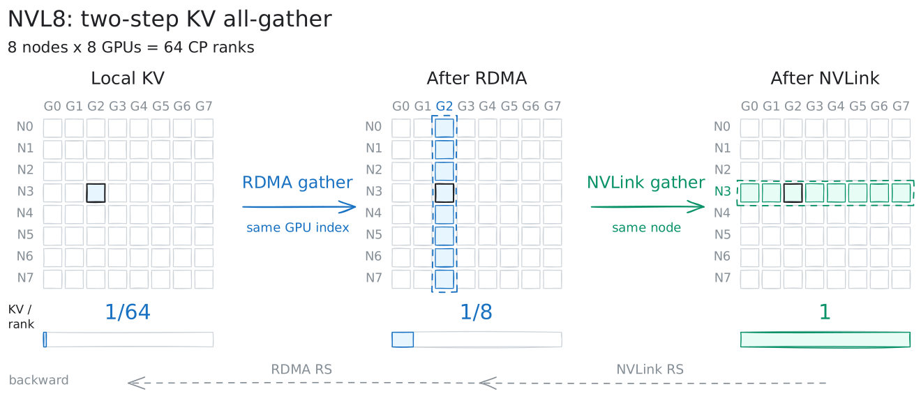
So let’s try two-dimensional CP. Assume CP=8*8=64.

With CP at 64, tokens per GPU drop to 1,048,576 / 64 = 16384
Latent KV per layer: (512 kv_lora + 64 rope + 128 indexer-K) * BF16 = 1408 B/token
At one million context, that’s 1.476 GB
One BF16 all-gather in the forward pass; one BF16 all-gather and one FP32 reduce-scatter in the backward pass.
The all-gather goes in two steps
1. RDMA: each GPU receives 1/64 of the KV from each of 7 GPUs on the other 7 nodes: 1.476 GB * 7/64 = 161.5 MB
2. NVLink: each GPU then receives 1/8 of the KV from each of the 7 GPUs on the same node: 1.476 GB * 7/8 = 1.292 GB
The reduce-scatter is similarly two steps, NVLink first and then RDMA.
Compared with CP64 on NVL72, the extra RDMA communication time for CP64 on NVL8 is 161.5 MB * (1 + 1 + 2) / 90 GB/s = 7.2 ms
Still assuming attention time at one million context is 4x the linear layers, one layer’s compute time is 4 GFLOP/token * 16384 token * (1 + 4) / (2.5 PFLOP/s * 80%) = 164 ms
Note that this 7.2 ms is on the critical path and cannot be hidden, equivalent to paying an extra 4.4% in time.
(2.5 PFLOP/s * 80%) * 122 ms / (4 GFLOP * (1 + 4)) = 12200 < 16384

So if this 2D CP is implemented well, one-million-token context can be done at a 4.4% time premium over NVL72. We also overestimated compute above, and therefore overestimated the communication overhead, so in practice it should be even lower.

Summary

After a long detour, what’s left is really just three things: FSDP, CP, EP.

This isn’t to say PP and TP are inherently sinful, or that Megatron is bad. Quite the opposite: Megatron grew into what it is today precisely because it has to support all kinds of models, all kinds of machines, and all kinds of parallelism combinations. Taken individually, every feature probably has a reason it absolutely must be added. It’s just that when all those reasons stack up, the result is Megatron. I have nothing but deep respect for teams that can maintain systems this complex.

But if we constrain the problem first, things look rather different.

NVL72 gives a huge high-speed communication domain, so EP and CP can stay inside NVLink; MoE stuffs the vast majority of parameters into experts, so the only troublesome thing across communication domains is sharding the expert weights; and long context itself provides enough compute to hide cross-node eFSDP communication behind it. So PP no longer has a reason to exist, and TP goes from mandatory to “add it once measurements show a gain”.

Even on machines with only NVL8, the same line of thinking keeps going: if NVLink isn’t enough, split CP into two dimensions and pay a bit of unhideable RDMA communication. RDMA bandwidth going up to 800 Gbps further makes this extra communication overhead easy to bear.

Only when a man has things he will not do can he accomplish things.

—— Mencius, Li Lou II

Building systems is probably like this too. You can always find a reason to add a feature; what’s genuinely hard is knowing what you can leave undone, and which complexity to refuse.

How not to build the next Megatron? Maybe the answer isn’t learning more forms of parallelism, but, after learning them all and doing the math, having the confidence to say:

Not this one.