Recently, the center of my work shifted from building inference systems to building post-training systems. Watching code that was clean and crisp in the inference engine turn into twists and turns inside the training framework, the furrow between my brows grew deeper. It runs slowly, it is inflexible to use, it is riddled with traps, and it is hard to maintain. This training framework was meant to be a lean system, yet it was drifting toward Megatron-level complexity.

My colleagues and I attempted refactors several times, but there was always some grime in the way of making the code elegant. Gradually, more and more clues pointed in the same direction: pipeline parallelism (PP).

Problems Brought by Pipeline Parallelism

Bubbles and Tuning

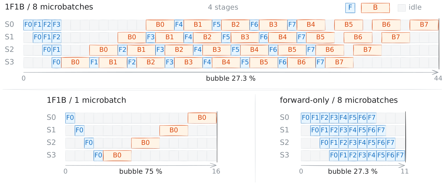
As everyone knows, the very structure of pipeline parallelism introduces bubbles. The entire field of machine learning systems is filled with stories of countless researchers wrestling with bubbles.

GPipe: the pioneering work, which splits the batch into multiple microbatches.
PipeDream: 1F1B, but it introduced the problem of mixing old and new weight versions (somewhat off-policy).
PipeDream-Flush: fixed 1F1B.
Interleaved 1F1B: slice the stages finer, so each rank holds several stages.
TeraPipe: within a microbatch, cut once more along the sequence dimension.
Zero Bubble: split dgrad and wgrad apart.
DualPipe: hide the EP communication over RDMA as much as possible.
(and many more)

Just understanding and implementing each of these algorithms already takes considerable effort.

Then, for every model, hardware, and dataset, you have to tune again. How many stages to cut into, how many microbatches. The head and tail of the model have different amounts of compute from the middle, so you also have to tune how many layers each stage gets. If there are multimodal inputs, those have to be pulled out and handled separately too.

If you don’t want to brute-force it or try configurations one by one on a hunch, tuning the parameters of a training framework is itself a deep discipline. How to estimate the overall runtime from profiling data of individual components, how to define the search space, how to model it as an algorithmic problem, how to solve the NP-hard planning problem, how to build a simulator… Research work keeps pouring out: DAPPLE, Piper, Alpa, Galvatron, nnScaler, Metis, Zorse, SimAI, Charon…

The Dynamics of Post-Training

All of the above still assumes that the input length and count are fixed. If we consider post-training, especially the needs of reinforcement learning post-training, things get even more complicated, because both the input length and the input count are dynamic, and in some cases the amount of data may even be very small. Pipeline parameters tuned for one input distribution may turn out worse under another.

In torchtitan, the pipeline schedule is fixed when the trainer starts: how many microbatches a round contains, when each stage computes and communicates, and how many copies of intermediate state need to be prepared are all constrained by one fixed schedule. Post-training inputs are not necessarily that regular, though. The number of microbatches a given step ends up cutting into may just barely exceed the schedule’s capacity. The extra inputs can’t be stuffed into the already-arranged pipeline; they can only go in another round.

Worse still, the overflow may be tiny. In the extreme case it is a single microbatch, which means the overflow round has an extremely high bubble ratio.

So people once again start patching up RL training systems: fusing schedules into the pipeline bubbles (RLHFuse), making generation and training asynchronous (PipelineRL, StreamRL), rearranging long-tail rollouts (RollPacker)…

Forward-Only Passes

In post-training, some algorithms require additional forward-only computation. On-policy Distillation and On-policy Self-distillation both introduce an extra forward pass of a teacher or reference model; algorithms like Importance Sampling and IcePop also make a single update contain compute stages with different numerical semantics and dependencies.

Note that the bubble ratio of a forward-only pass is just as large as that of 1F1B. If you naively add the extra forward-only computation, that amounts to adding even more bubbles. And if you want to merge these extra forward-only passes with the model’s normal forward and backward passes, then you need a pipeline-parallel schedule designed specifically for each algorithm.

Sequence Padding

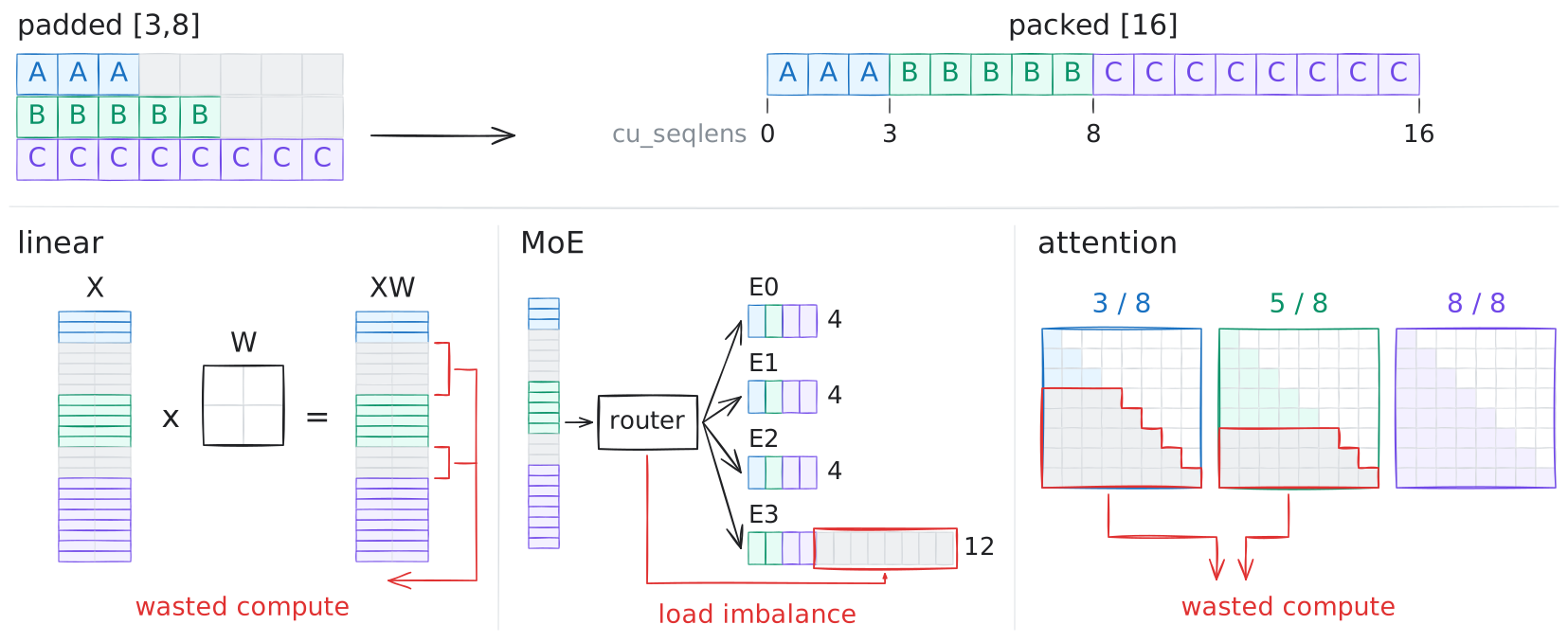
When I first started reading the training framework’s code, the thing I could least understand was why the input had to be padded into a [B, S] shape rather than simply being a [T]. Back in 2022, Orca already told everyone that there’s no need to pad; just concatenate all the sequences together. My blog post from 2023 also explained how to derive this conclusion from first principles. Yet in 2026, for training frameworks, sequence padding is still the standard, and flattening and concatenating has instead become an advanced optimization called Packed Sequences, Sequence Packing, or THD, with plenty of restrictions attached. Mind you, over on the inference side, no inference engine would have the nerve to advertise support for continuous batching as a selling point, with fine print underneath: not all models support this feature, not all configurations are compatible with this feature, enabling this feature conflicts with many other features; experimental, enable with caution.

Inelegant

Why don’t I like sequence padding? Mainly because it is not a hard constraint at all.

Throughout the model’s computation, apart from the attention mechanism, which operates on the concept of a “sequence”, every other part operates directly on tokens. And the attention operator itself supports irregular inputs, such as varlen in FlashAttention. In the spirit of Occam’s razor, “do not multiply entities beyond necessity,” deliberately padding [T] into [B, S] is an inelegant thing to do.

My preference is that if something is standing in the way of flattened inputs, that problem should be solved locally, rather than letting padding become a global requirement.

Waste, and Reducing Waste

Once padding is introduced, useless computation inevitably follows. Then, to minimize this waste, people patch things up here and there.

In MoE, these padding tokens may all get thrown at the same expert, causing severe load imbalance. Megatron has an optimization where the MoE router accepts a padding_mask, so that padding tokens can be skipped. Ingenious!

…But on second thought, if we hadn’t padded the tokens in the first place, this optimization would have no reason to exist.

torchtune / torchtitan / FlexAttention

torchtune once adopted an approach to padding that made my eyes light up like nothing else. The following very well-written docstring accurately illustrates that design:

class PackedDataset(Dataset):
    """
    Performs greedy sample packing on a provided dataset.

    (...)

    A packed sample is made up of individual smaller sequence length samples jammed together
    within ``max_seq_len``. For example, if max_seq_len is 6 and there are varied
    length samples::

        tokens = [
            [S1, S1, S1, S2, S2, pad],
            [S3, S3, S4, S4, pad, pad],
            ...,
        ]

    To prevent cross-contamination, the following mask would be returned for the
    first pack in the example::

        mask = [
            [1, 0, 0, 0, 0, 0],
            [1, 1, 0, 0, 0, 0],
            [1, 1, 1, 0, 0, 0],
            [0, 0, 0, 1, 0, 0],
            [0, 0, 0, 1, 1, 0],
            [0, 0, 0, 0, 0, 1],
        ]

    The position ids would be::

        input_pos = [
            [0, 1, 2, 0, 1, 2],
            [0, 1, 0, 1, 2, 3],
            ...,
        ]

After copying this docstring, I was stun-locked for another ten minutes, because what this class does is truly out of this world.

It increases the algorithmic complexity.
- Let each sequence have length \(s_i\), with \(b\) sequences in total, \(M\) the packed length, and \(n\) the number of rows after this code finishes packing.
- The complexity of attention should be \(\Theta\!\left(\sum_{i=1}^{b} s_i^2\right)\).
- After this code’s treatment, it shoots straight up to \(\Theta(n M^2)\).
- Worst case: suppose \(s_i = 1\) and \(b = M\). The complexity should be \(\Theta\!\left(\sum_{i=1}^{M} 1^2\right) = \Theta(M)\), but now it becomes \(\Theta\!\left(\frac{\sum_{i=1}^{M} 1}{M} \cdot M^2\right)=\Theta(M^2)\). A qualitative change!
- Taking a step back, suppose \(s_i = s\) and \(M = k s\), so each row holds \(k\) sequences. The complexity should be \(\Theta(bs^2)\), but now it becomes \(\Theta\!\left( \frac{b}{k}(ks)^2 \right) = \Theta(bs^2 k)\), a degradation by a factor of \(\Theta(k)\).
It constructs an \(M^2\) attention mask.
- This genuinely occupies \(M^2\) of GPU memory.
- It also genuinely adds \(M^2\) of memory traffic.
- Mind you, ever since FlashAttention was invented in 2022, the extra space can grow linearly with the number of tokens rather than quadratically with the sequence length.
It writes more code to make the program slower and use more memory.
- The packing alone is already quite a hassle, and then you also have to carefully get the construction of the block-diagonal matrix right.
- Without padding, you just concatenate all the tokens, record cu_seqlens along the way, and pass is_causal=True to the attention operator. Done.

Evidently the torchtune developers realized this too, so in PR 1193 they introduced FlexAttention and torch.compile, for a straight 1.4x speedup. torchtune’s packing scheme was also carried over into torchtitan, where it became FirstFitPackingConfig.

Even if the performance can catch up, I still don’t much like this scheme:

Using FlexAttention + torch.compile to quickly implement all sorts of novel attention mechanisms is a great approach, but using it for regular attention is a bit like using an anti-aircraft gun to swat a mosquito.
The performance guarantee has effectively been offloaded into the complexity of FlexAttention and torch.compile.
You still have to write complex packing code and construct the equivalent block-diagonal structure, get_efficient_causal_mask_mod_for_packed_document; it’s just that now it is compilable structured metadata rather than a real dense matrix.
It still sounds inelegant, like a patch on top of a patch.

Error-Prone

In 2024, Unsloth found a loss calculation bug in Transformers. The cause was that during gradient accumulation, each microbatch’s own mean loss was averaged with equal weights rather than weighted by the number of valid tokens. Padding makes the number of valid tokens uneven across microbatches, and that equal-weight average went wrong. Megatron has fixed the same problem as well.

-    loss = F.cross_entropy(logits, labels, ignore_index=-100)
+    loss = F.cross_entropy(logits, labels, ignore_index=-100, reduction="sum")
+    loss = loss / num_tokens

If you don’t use padding, and instead let the input length directly reflect the true number of valid tokens, then when designing the loss it becomes hard to dodge one question: should the loss be averaged per token, or per sequence? Whichever you choose, at least it is an explicit design decision.

This bug arises easily because in fixed-length pretraining, the number of valid tokens in every sequence and every microbatch is usually the same. In that case, “average within each microbatch, then average across them” and “put all tokens together and average” happen to be equivalent, so the distinction stayed hidden for a long time. Come post-training, sequence lengths differ, the number of valid tokens per padded microbatch differs too, and carrying over the old reduction is simply wrong.

Similarly, NVIDIA’s article this year also mentioned a bug caused by forgetting to subtract padding tokens:

Previous versions of Megatron Core didn’t account for the THD layout and assumed max_seqlen is the effective sequence length when computing FLOPs. Leading to systematic overestimation in variable-length scenarios.

Same principle as before: if the data structure directly expressed the true number of valid tokens from the start, this class of bugs would at least be harder to hide.

Static Shapes

Sequence padding, of course, was not invented for pipeline parallelism; data loaders and kernels share the blame. But for it to have grown, over the long run, from a local implementation choice into a global shape contract for the entire training stack, pipeline parallelism must bear responsibility.

Megatron’s ModelParallelConfig and pipeline_parallel/schedules.py both point out that with pipeline parallelism, you had better use a fixed [B, S], otherwise there is a performance penalty:

# https://github.com/NVIDIA/Megatron-LM/blob/f2f0f7bfd88fcb1243df55275988d6af52daea35/megatron/core/model_parallel_config.py#L385-L389
class ModelParallelConfig:
    ###################
    # Pipeline Parallel
    ###################
    variable_seq_lengths: bool = False
    """Support for variable sequence lengths across microbatches. Setting this communicates the size
        of tensors during pipeline parallelism communication, because of this extra overhead it
        should only be set if the sequence length varies by microbatch within a global batch.
    """

# https://github.com/NVIDIA/Megatron-LM/blob/f2f0f7bfd88fcb1243df55275988d6af52daea35/megatron/core/pipeline_parallel/schedules.py#L116-L121
def get_forward_backward_func(...):
    """
    seq_length (int, required): Sequence length of the current global batch. If this is a dual-stack
        transformer, this is the encoder's sequence length. This is ignored if variable_seq_lengths
        in the config is True. Otherwise, each microbatch in the current global batch size must use
        this sequence length.

    micro_batch_size (int, required): The number of sequences in a microbatch.

    """

The torch.distributed.pipelining documentation states explicitly that input shapes must be static:

A PipelineStage needs to know the input and output shapes for the stage model, so that it can correctly allocate communication buffers. The shapes must be static, e.g. at runtime the shapes can not change from step to step.

In addition, PyTorch automatically chunks the whole batch into microbatches:

# https://github.com/pytorch/pytorch/blob/v2.13.0/torch/distributed/pipelining/schedules.py#L505-L527
class _PipelineSchedule(ABC):
    @abstractmethod
    def step(
        self,
        *args,
        target=None,
        losses: list | None = None,
        return_outputs=True,
        loss_kwargs: dict[str, Any] | None = None,
        **kwargs,
    ):
        """
        Run one iteration of the pipeline schedule with *whole-batch* input.
        Will chunk the input into microbatches automatically, and go through the
        microbatches according to the schedule implementation.

        args: positional arguments to the model (as in non-pipeline case).
        kwargs: keyword arguments to the model (as in non-pipeline case).
        target: target for the loss function.
        losses: a list to store the losses for each microbatch.
        return_outputs: whether to return the outputs from the last stage.
        loss_kwargs: extra keyword arguments forwarded to the loss function.
        """

Obviously, without the B dimension, this chunking can’t happen.

For pretraining, static-shape inputs are understandable, but for post-training, static shapes become a rigid restriction.

Implementation Flaw or Fundamental Limitation?

Honestly, I don’t quite understand why Megatron’s and PyTorch’s pipeline parallelism require fixed input shapes. In my view, this restriction shouldn’t be fundamental; it looks more like an implementation flaw, or a design that wasn’t thought through.

First, the automatic microbatch chunking: yes, without B you can’t chunk automatically. But that doesn’t mean you can’t chunk manually. You can construct each microbatch’s cu_seqlens by hand and slice the input sequences by hand.

Second, the communication buffers mentioned in the PyTorch docs. As I understand it, allocating a buffer doesn’t need to care whether the shape is two-dimensional [B, S] or flattened to one-dimensional [T], nor whether [T] is variable. As long as T has an upper bound, allocate according to that bound and you’re done. Yet both PyTorch and Megatron require fixed-size buffers to accommodate the limitations of the NCCL send/recv API.

As I mentioned in a previous blog post and in the fabric-lib paper at MLSys 2026, RDMA, whether two-sided SEND/RECV or one-sided WRITE or READ, has no requirement that buffer sizes match on both ends; the buffer only needs to be large enough. On the other hand, communication over NVLink is based on memory semantics and likewise doesn’t require both parties to have the same buffer size. So this restriction comes from the NCCL API, and it is not fundamental.

Why does the docstring for Megatron’s variable_seq_lengths say that dynamic lengths carry a large performance penalty? I took a quick look at the pipeline-parallel implementation, and there are two obvious reasons:

# https://github.com/NVIDIA/Megatron-LM/blob/f2f0f7bfd88fcb1243df55275988d6af52daea35/megatron/core/pipeline_parallel/p2p_communication.py
# Simplified
class P2PCommunicator:
    def _communicate_shapes(self, ...):
        if is_sender:
            send_prev_shape_tensor = torch.tensor(tensor_send_prev.size(), ...)
            send_next_shape_tensor = torch.tensor(tensor_send_next.size(), ...)
            send_prev_op = P2POp(isend, send_prev_shape_tensor, self.prev_rank, self.pp_group)
            send_next_op = P2POp(isend, send_next_shape_tensor, self.next_rank, self.pp_group)
            ops = [send_prev_op, send_next_op]
        else:
            recv_prev_shape_tensor = torch.empty((3,), ...)
            recv_next_shape_tensor = torch.empty((3,), ...)
            recv_prev_op = P2POp(irecv, recv_prev_shape_tensor, self.prev_rank, self.pp_group)
            recv_next_op = P2POp(irecv, recv_next_shape_tensor, self.next_rank, self.pp_group)
            ops = [recv_prev_op, recv_next_op]

        work_list = torch.distributed.batch_isend_irecv(ops)  # submit to cuda stream
        for work in work_list:
            work.wait()  # cuda stream wait (non blocking)

        if is_sender:
            return [0, 0, 0], [0, 0, 0]
        recv_prev_shape = recv_prev_shape_tensor.tolist()  # block on D2H
        recv_next_shape = recv_next_shape_tensor.tolist()  # block on D2H
        return recv_prev_shape, recv_next_shape

    def _communicate(self, ...):
        # shape
        if config.variable_seq_lengths:
            recv_prev_shape, recv_next_shape = self._communicate_shapes(...)
        else:
            recv_prev_shape, recv_next_shape = tensor_shape, tensor_shape

        # payload
        if is_sender:
            send_prev_op = P2POp(isend, tensor_send_prev, self.prev_rank, self.pp_group)
            send_next_op = P2POp(isend, tensor_send_next, self.next_rank, self.pp_group)
            ops = [send_prev_op, send_next_op]
        else:
            tensor_recv_prev = torch.empty(recv_prev_shape, ...)
            tensor_recv_next = torch.empty(recv_next_shape, ...)
            recv_prev_op = P2POp(irecv, tensor_recv_prev, self.prev_rank, self.pp_group)
            recv_next_op = P2POp(irecv, tensor_recv_next, self.next_rank, self.pp_group)
            ops = [recv_prev_op, recv_next_op]
        work_list = torch.distributed.batch_isend_irecv(ops)
        if is_sender:
            return None, None, work_list
        return tensor_recv_prev, tensor_recv_next, work_list

Before every point-to-point communication, an extra communication is needed to obtain the shape information.
After submitting the shape-information communication, it calls .tolist(). This brings two more problems: first, it triggers a D2H transfer; second, the CPU control flow is blocked on this D2H transfer, which in effect means it is blocked on the shape-information communication.

Implemented this way, the performance loss is no small matter. But is it really necessary to implement it this way?

For pipeline parallelism, before each microbatch enters the pipeline, its token count and the shapes of the hidden states to be passed between stages can already be determined. Unlike expert parallelism (EP), where they change at every layer, there is no need to wait until each stage-to-stage transfer to ask on the spot.

Seen this way, these static-shape restrictions of pipeline parallelism are all just implementation problems, not fundamental requirements of the pipeline algorithm.

Recent Upstream Fixes

Interestingly, while I was writing this article, upstream happened to fix several of the problems mentioned above.

pytorch PR 188500 Allow explicit pre-split pipeline microbatches: adds arg_mbs, kwarg_mbs, and target_mbs to schedule.step(), allowing the caller to pre-split the microbatches before passing them in, no longer forcing the scheduler to chunk along dim 0 for you. This way we can construct each microbatch’s cu_seqlens ourselves.
torchtitan PR 3856 Always Pre-Split Microbatches for PP: moves the responsibility for splitting microbatches to the data loader, lets the data loader construct the microbatch inputs, and removes the “PP is incompatible with varlen” restriction.
torchtitan PR 4121 fold batch dim: switches the entire data path from [B, S] to [T], and changes the configuration from being expressed in number of sequences to a per-DP-rank, per-microbatch token budget.

These fixes confirm my earlier judgment about static shapes: [B, S], automatic microbatch chunking along dim 0, and PP being mutually exclusive with varlen are none of them fundamental limitations of pipeline parallelism, but API choices and implementation flaws.

To fix this local restriction, ownership of microbatches moved from the scheduler to the data loader, and the trainer, validator, TorchFT, Forge, and tests all had to change along with it; concepts like checkpoint interval, originally expressed in data-loader steps, also had to be reinterpreted. The elements of arg_mbs and kwarg_mbs are still Any, and the model input type still can’t pass through schedule.step() and get statically checked. The model is still split into model_parts, different stages still receive inputs with different semantics, and only the last stage produces a real loss.

Fixing some of the historical baggage is of course worth celebrating, but note that these fixes still pull one thread and move the whole body. Pipeline parallelism can certainly be implemented the right way; the problem is that to get it right, the entire framework has to participate, and every component of the framework needs to understand the concept of pipeline parallelism. This is the maintenance price you are forced to pay for using pipeline parallelism.

Engineering Burden

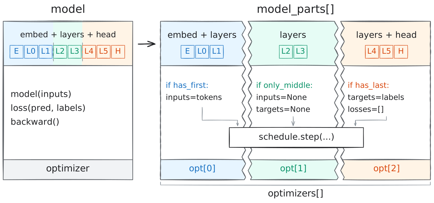
Setting aside the engineering effort pipeline parallelism itself requires, pipeline parallelism also imposes a great deal of extra engineering burden on every other part of the training framework. Here I’ll mainly use torchtitan as the example.

Control-Flow Forks

Once pipeline parallelism is enabled, a lot of control flow becomes completely different from when it is off. To unify the two as much as possible, the normal path often gets complicated too.

Take the most central pieces, model construction and the single-step forward-backward pass. Even written as over-simplified pseudocode, you can see a large number of control-flow forks. You can even see a fake loss being returned just to keep the interface consistent. And similar patterns repeat across multiple components.

# https://github.com/pytorch/torchtitan/blob/4c6481182c1c3d7815e3a119a271eebead94c71a/torchtitan/trainer.py
# Over-simplified
class Trainer:
    def __init__(self, ...):
        model = model_spec.model(config.model)  # on meta device

        # Fork: how model inits
        if parallel_dims.pp_enabled:
            pp_schedule, model_parts, pp_has_first_stage, pp_has_last_stage = \
                model_spec.pipelining_fn(model, ...)
            del model
            for m in model_parts:
                m.to_empty(device)
                cast(BaseModel, m).init_weights()
                m.train()
            ensure_pp_loss_visible(parallel_dims, pp_schedule_name)
        else:
            pp_schedule, pp_has_first_stage, pp_has_last_stage = None, None, None
            model = model_spec.parallelize_fn(model, ...)
            model.to_empty(device)
            cast(BaseModel, model).init_weights()
            model.train()
            model_parts = [model]
        
        # Fork: where lm_head lives
        if isinstance(loss_fn, ChunkedLossWrapper):
            if parallel_dims.pp_enabled:
                if pp_has_last_stage:  # lm_head in PP last stage
                    loss_fn.set_lm_head(model_parts[-1].lm_head)
                    model_parts[-1]._skip_lm_head = True
                else:
                    pass  # non-last stage: no lm_head
            else:
                # lm_head in the only model part
                assert len(model_parts) == 1
                loss_fn.set_lm_head(model_parts[0].lm_head) 
                model_parts[0]._skip_lm_head = True
                

    def forward_backward_step(self, ...):
        # Fork: model forward + backward vs schedule step
        if parallel_dims.pp_enabled:
            with train_context():
                # Fork: stage-dependent args passed to schedule step
                if pp_has_last_stage:
                    targets, losses = labels, []
                else:
                    targets, losses = None, None

                if pp_has_first_stage:
                    pp_schedule.step(inputs, target=targets, losses=losses, ...)
                else:
                    pp_schedule.step(        target=targets, losses=losses, ...)

            # Fork: stage-dependent loss computation
            if pp_has_last_stage:
                assert losses is not None
                loss = sum(stack(losses)).to(device)
            else:
                loss = tensor([-1.0], device=device)  # fake value

        else:
            assert len(model_parts) == 1
            with train_context():
                pred = model_parts[0](inputs, ...)
                loss, _ = loss_fn(pred, labels, ...)
                loss.backward()
        return loss


class Validator:
    def validate(self, model_parts, ...)
        # Fork patterns similar to forward_backward_step

Beyond the control-flow forks, the forward_backward_step above is itself quite a delicate piece. Notice that it checks the pipeline-parallel stage multiple times, which looks awfully convoluted. Isn’t this just giving different inputs and outputs depending on whether the current rank is in the first, middle, or last stage? Why not replace it with the simpler form below:

        if parallel_dims.pp_enabled:
            with train_context():
                if pp_has_first_stage:
                    pp_schedule.step(inputs, target=None,   losses=None,   ...)
                    loss = tensor([-1.0], device=device)
                elif pp_has_last_stage:
                    losses = []
                    pp_schedule.step(        target=labels, losses=losses, ...)
                    loss = sum(stack(losses)).to(device)
                else:
                    pp_schedule.step(        target=None,   losses=None,   ...)
                    loss = tensor([-1.0], device=device)
        else:
            ...

In fact, once you take VPP into account, this code is wrong, because with VPP enabled a single rank may own multiple stages.

Model Surgery

After constructing the entire model on the meta device, torchtitan prunes the model object according to the pipeline stage. Put charitably, this makes full use of the dynamic nature of the Python language. But in my view, this kind of dynamic manipulation is extremely fragile and error-prone; every time I see a setattr I break into a sweat.

# https://github.com/pytorch/torchtitan/blob/4c6481182c1c3d7815e3a119a271eebead94c71a/torchtitan/distributed/pipeline_parallel.py#L428
# simplified

def _split_module(whole_model: nn.Module, modules_to_keep: set[str]) -> nn.Module:
    model = copy.deepcopy(whole_model)
    for name, m in model.named_children():
        if isinstance(m, (nn.ModuleDict, nn.ModuleList)):
            layers_to_keep: set[str] = ...
            if layers_to_keep:
                # Keep only specified layers
                if isinstance(m, nn.ModuleDict):
                    for layer_name in list(m.keys()):
                        if layer_name not in layers_to_keep:
                            del m[layer_name]
                elif isinstance(m, nn.ModuleList):
                    indices_to_keep: list[int] = ...
                    new_layers = nn.ModuleList([
                        l for i, l in enumerate(m) if i in indices_to_keep])
                    setattr(model, name, new_layers)
            else:
                # No layers from this structure needed, set to empty structure
                if isinstance(m, nn.ModuleDict):
                    setattr(model, name, nn.ModuleDict())
                elif isinstance(m, ModuleList):
                    setattr(model, name, nn.ModuleList())
        elif name not in modules_to_keep:
            # Replace with None
            setattr(model, name, None)
    return model

After this round of pruning, some submodules may become None, and the model’s forward definition becomes complicated and muddled:

# https://github.com/pytorch/torchtitan/blob/4c6481182c1c3d7815e3a119a271eebead94c71a/torchtitan/models/common/decoder.py#L262
# simplified
class Decoder(BaseModel):
    """Base class for autoregressive decoder-only language models."""

    def forward(self, tokens: torch.Tensor, ...):
        # Note: `tokens` is int token ids in the first stage,
        # but becomes hidden states in later stages.
        if self.tok_embeddings is not None:
            h = self.tok_embeddings(tokens)
        else:
            h = tokens

        # Note: all stages happen to have an iterable `layers`.
        for layer in self.layers.values():
            h = layer(h, ...)

        # Note: only last stage has `norm`.
        if self.norm is not None:
            h = self.norm(h)
        
        # Note: only last stage has `lm_head`
        if self.lm_head is not None:
            output = self.lm_head(h)
        else:
            output = h

        # Note: `output` is hidden states in earlier stages,
        # but becomes logits in the last stage.
        return output

What was a plain and simple forward now has to check is not None at every single step. And just from reading this code, you can’t tell which modules are supposed to appear in which stages.

The inputs and outputs are muddled too. The input parameter tokens sounds like token IDs, but in later stages it is actually hidden states. output is hidden states in earlier stages, and logits in the last stage.

Concept Leakage

Other parts of the training framework need special adaptation for pipeline parallelism. A few examples:

What used to be a single model object is now a model_parts list.
Similarly, CheckpointManager, Optimizer, and LRScheduler all went from a single object to a series of objects.
set_determinism originally only needed to set the same random seed on all ranks, but with pipeline parallelism enabled, ranks in different stages need different random seeds.
clip_grad_norm_ needs to handle pipeline parallelism separately, because pipeline parallelism deletes part of the parameters on each rank.
MetricsProcessor needs to know the pipeline-parallel schedule.

The Type System Stops Working

The examples above already reflect many scenarios where static type checking loses its power:

Dynamic operations like setattr are certainly not protected by static checking.
Because of the control-flow forks, many variables become nullable.
One object becomes a list of objects.
After being split by pipeline parallelism, what was a Decoder type or a BaseModel base class becomes list[nn.Module], losing the interface the base class had. So later on, cast(BaseModel, ...) and cast(Decoder, ...) are used to get the corresponding functionality back. No type-system guarantee whatsoever.

Granted, some of these problems are purely torchtitan’s own. But when we were improving type checking in our training framework earlier, we ran into one thing that simply can’t be done as long as you use torch.distributed.pipelining.

At the time, I mainly wanted to improve the abstract method Model.forward of the Model abstract class.

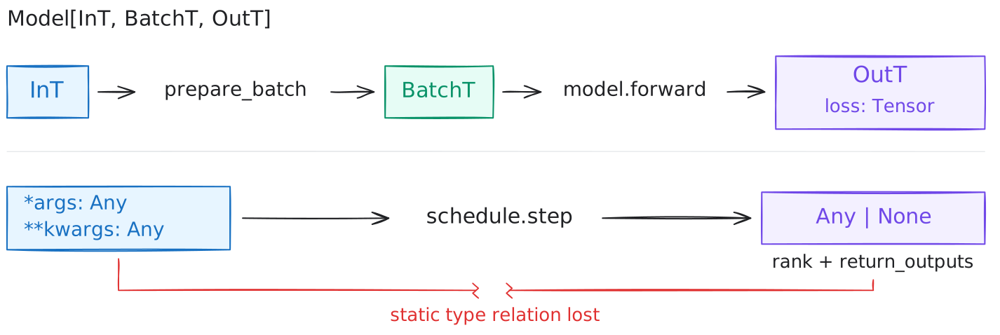
A task generally has a data loader that produces inputs related to that task. Let’s call this type InT.
The task corresponds to a specific model wrapper, which generally inherits from a concrete model architecture. Let’s call the type of this model wrapper Model.
Each Model expects different batch input tensors. Let’s pack all the tensors into a BatchT type.
Each Model also knows how to convert an InT into a BatchT. Let’s call this function prepare_batch.
Each Model’s output may also differ. Let’s call it OutT. Since we need backpropagation, we require every OutT to contain a loss tensor.

Obviously, every concrete Model implementation knows exactly what its own InT, BatchT, and OutT are. In Rust, using Associated Types, we can define a generic interface like this:

pub trait ModelOutput {
    fn loss(&self) -> Tensor;
}

pub trait Model {
    type In;
    type Batch;
    type Output: ModelOutput;
    fn prepare_batch(&self, inputs: Self::In) -> Self::Batch;
    fn forward(&mut self, batch: Self::Batch) -> Self::Output;
}

In Python, although there are no associated types, we can simulate this behavior with Generics:

class ModelOutput(Protocol):
    @property
    def loss(self) -> Tensor: ...

class Model[InT, BatchT, OutT: ModelOutput](ABC):
    @abstractmethod
    def prepare_batch(self, inputs: InT) -> BatchT: ...

    @abstractmethod
    def forward(self, batch: BatchT) -> OutT: ...

Then consider the rough flow of Trainer.step(). Basically it reads the next chunk of data, converts it, and then runs forward and backward. Notice that the Trainer itself doesn’t actually care about the concrete type at each of these steps, as long as they line up with each other. With the abstraction above, we can write the following code that passes type checking:

class Trainer[InT, BatchT, OutT: ModelOutput]:
    loader: Iterator[InT]
    model: Model[InT, BatchT, OutT]

    def step(self) -> OutT:
        inputs = next(self.loader)
        batch = self.model.prepare_batch(inputs)
        out = self.model.forward(batch)
        out.loss.backward()
        return out

This way we can guarantee that even if the Trainer implementation gets complicated, or the Model’s input changes, static type checking will catch the inconsistencies.

Unfortunately, if you use PyTorch’s pipeline-parallel implementation, this lovely type system can’t be used. self.model.forward() has to be replaced with pp_schedule.step().

First, as mentioned earlier, pp_schedule.step() automatically splits microbatches, so it requires the arguments passed in to be individually listed Tensors. Obviously, passing in a dataclass here won’t fit.

Second, pp_schedule.step() erases the type information with args and kwargs (see the code pasted in the earlier section). As a result, even simple mistakes like a missing argument or a misspelled argument name can’t surface until runtime.

PP=1

You might say: suppose I don’t plan to use pipeline parallelism; then I can just set PP=1. Is it really necessary to delete the code?

It’s true that with PP=1, many of the performance shortfalls and functional restrictions may be lifted. But I still think that if there is no plan to use pipeline parallelism, the code should be deleted.

If you stop maintaining the pipeline-parallel code, that part of the control flow will gradually rot. When one day in the future you actually want to use pipeline parallelism, it may no longer run correctly.
If you decide to keep maintaining the pipeline-parallel code, you pay a high maintenance and development cost, because what you are maintaining is not just the pipeline-parallel code itself. For every new feature and every patch, you have to spend more time designing and more time implementing to ensure the change is compatible with pipeline parallelism.
Even with the help of coding agents, designing and implementing new code is still harder than it would be with the pipeline-parallel code deleted. This isn’t because we humans aren’t smart enough or because the agents aren’t capable enough, but because the problem space has grown. Once a new feature introduces a new execution path, as pipeline parallelism does, the number of combinations of all features grows exponentially, and every one of those combinations is a code path that needs to be tested and maintained.

When Pipeline Parallelism Is Still the Right Answer

I have been bashing pipeline parallelism throughout this article, but here I’ll also say a few fair words on its behalf.

If the scale-up domain doesn’t have enough memory and the scale-out domain is slow, then pipeline parallelism still has a performance advantage.

For example, Hopper-generation NVLink generally only interconnects 8 GPUs, and the accompanying RDMA is generally at most 400 Gbps per GPU. Under those conditions, if you want to train a trillion-parameter model and also support million-token context, pipeline parallelism is the most direct approach. This also explains why most model reports so far use pipeline parallelism: NVL72, B300, and 800 Gbps RDMA haven’t been rolled out at scale for very long.

On the other hand, using pipeline parallelism for pretraining is also reasonable. After all, pretraining has fixed input shapes and large data volumes, so fairly high performance can be reached even with pipeline parallelism.

Summary

This article laid out the problems of pipeline parallelism from two angles: performance tuning and engineering complexity.

Among the various forms of parallelism, pipeline parallelism is the odd one out. Other parallelism schemes also shard parameters, activations, and data, and introduce communication and even local control flow, but they largely preserve the model’s original execution structure; the performance discussion is mainly about whether compute can be accelerated and whether communication can be hidden behind compute. Pipeline parallelism, however, cuts the computation graph open along the layers and globally rewrites the control flow of the entire forward and backward pass. The result is that its concepts leak all the way into every corner of the training framework. Pipeline parallelism itself also doesn’t speed up compute. To save memory and reduce communication volume, the price it pays is extra scheduling complexity and structural waste in the form of pipeline bubbles.

Considering new hardware and post-training workloads, I decided to delete pipeline parallelism. Of course, I’m not just complaining in this article, digging a hole and walking away without filling it. In the next blog post, I will derive how to train without pipeline parallelism.