Paper Notes: Ad Click Prediction: a View from the Trenches
- Paper Link: https://www.eecs.tufts.edu/~dsculley/papers/ad-click-prediction.pdf
- Presentation Slides: https://courses.cs.washington.edu/courses/cse599s/14sp/kdd_2013_talk.pdf
In this paper:
- FTRL-Proximal online learning algorithm, which has excellent sparsity and convergence properties
- Improvement on the use of per-coordinate learning rates
- Some of the challenges that arise in a real-world system that may appear at first to be outside the domain of traditional machine learning research
- Memory saving
- Assessing and visualizing performance
- Providing confidence estimates for predicted probabilities
- Calibration methods
- Automated management of features
System overview
- Data tends to be extremely sparse.
- Although the feature vector x might have billions of dimensions, typically each instance will have only hundreds of nonzero values.
- We train a single-layer model rather than a deep network of many layers.
- This allows us to handle significantly larger data sets and larger models, with billions of coefficient.
- We are much more concerned with sparsity at serving time rather than during training because trained models are replicated to many data centers for serving
FTRL-Proximal
- Each training example only needs to be considered once.
- In practice another key consideration is the size of the final model; since models can be stored sparsely, the number of non-zero coefficients in
wis the determining factor of memory usage.- (My question: many zero coefficients in
wmean many dimension of the feature vector is useless? Why do we bother to have them?)
- (My question: many zero coefficients in
- Simply adding L1 penalty will essentially never produce coefficients that are exactly zero.
- FTRL-Proximal gives significantly improved sparsity with the same or better prediction accuracy.
- FTRL-Proximal: Follow The (Proximally) Regularized Leader
Instead of $w_{t+1} = w_t - \eta_t g_t$, the update rule for FTRL-Proximal is:
\[w_{t+1} = \underset{w}{\arg \min} \left( g_{1:t} \cdot w + \frac12 \sum_{s=1}^t \sigma_s \lVert w - w_s \rVert_2^2 + \lambda_1 \lVert w \rVert_1 \right)\]where
- $\eta_{t,i} = \frac{\alpha}{\beta + \sqrt{\sum_{s=1}^t g_{s,i}^2}}$
- $g_t$ is the gradient
- $g_{1:t} := \sum_{s=1}^t g_s$
- $\sigma_s = \sqrt{s} - \sqrt{s-1}$
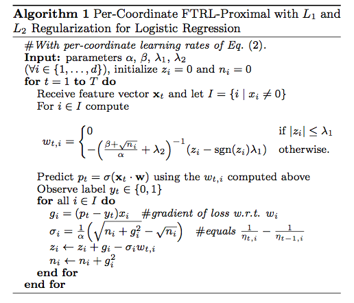
An interesting thing is $w_{t,i}$ can be solved in closed form, thus FTRL-Proximal only stores $z \in \mathbb{R}^d$ in memory. Here is the algorithm:
Another interesting thing is that when $\eta_t$ is a constant value $\eta$ and $\lambda_1 = 0$, it is easy to see the equivalence to online gradient descent.
Per-Coordinate learning rates
- At least for some problems, per-coordinate learning rates can offer a substantial advantage.
- A simple thought experiment: suppose we are estimating
Pr(heads | coin_i)for some coins using logistic regression.- We decrease the learning rate for coin i even when it is not being flipped. This is clearly not the optimal behavior.
- A careful analysis shows the per-coordinate rate $\eta_{t,i} = \frac{\alpha}{\beta + \sqrt{\sum_{s=1}^t g_{s,i}^2}}$ is near-optimal in a certain sense.
- The optimal value of $\alpha$ can vary a fair bit depending on the features and dataset, and $\beta = 1$ is usually good enough.
- (My question: Where do alpha and beta come from?)
Saving memory at training time
Probabilistic Feature Inclusion
- In many domains with high dimensional data, the vast majority of features are extremely rare.
- Probabilistic Feature Inclusion: new features are included in the model probabilistically as they first occur
- Poisson Inclusion: for a new feature, add with probability $p$.
- Bloom Filter Inclusion: use a rolling set of counting Bloom filter. Once a feature has occurred more than n times (according to the filter), add it to the model. (My question: Bloom filter?)
- Bloom filter approach gives a better set of tradeoffs for RAM savings against loss in predictive quality.
Encoding Values with Fewer Bits
- Nearly all of the coefficient values lie within the range (−2, +2). Analysis shows that the fine-grained precision is also not needed.
q2.13encoding: 16 bits per value: reserve two bits to the left of the binary decimal point, thirteen bits to the right of the binary decimal point, and a bit for the sign.- To reduce round-off error, do an explicit rounding: $v_{\text{rounded}} = 2^{-13} \left\lfloor 2^{13} v + R \right\rfloor$ where $R$ is a random deviate uniformly distributed between 0 and 1.
Progressive Validation
- Because computing a gradient for learning requires computing a prediction anyway, we can cheaply stream those predictions out for subsequent analysis, aggregated hourly.
- The online loss is a good proxy for our accuracy in serving queries, because it measures the performance only on the most recent data before we train on it –exactly analogous to what happens when the model serves queries.
- We therefore always look at relative changes, usually expressed as a percent change in the metric relative to a baseline model. In our experience, relative changes are much more stable over time.
- (My question: what exactly is progressive validation?)
(Sections I didn’t read carefully or cannot understand)
- 4.3: Training Many Similar Models
- 4.4: A Single Value Structure
- 4.5: Computing Learning Rates with Counts
- 4.6: Subsampling Training Data
- 5: Evaluating Model Performance
- 6: Confidence Estimates
- 7: Calibrating Predictions
- 8: Automated Feature Management
- 9: Unsuccessful Experiments