Dissecting Batching Effects in GPT Inference
Machine learning models relying on batching to improve inference throughput, especially for smaller computer vision models such as ResNet and DenseNet. GPT, as well as other large language models (LLMs), is the hottest model these days. Does batching still apply to GPT and LLMs? Let’s find out.
Background
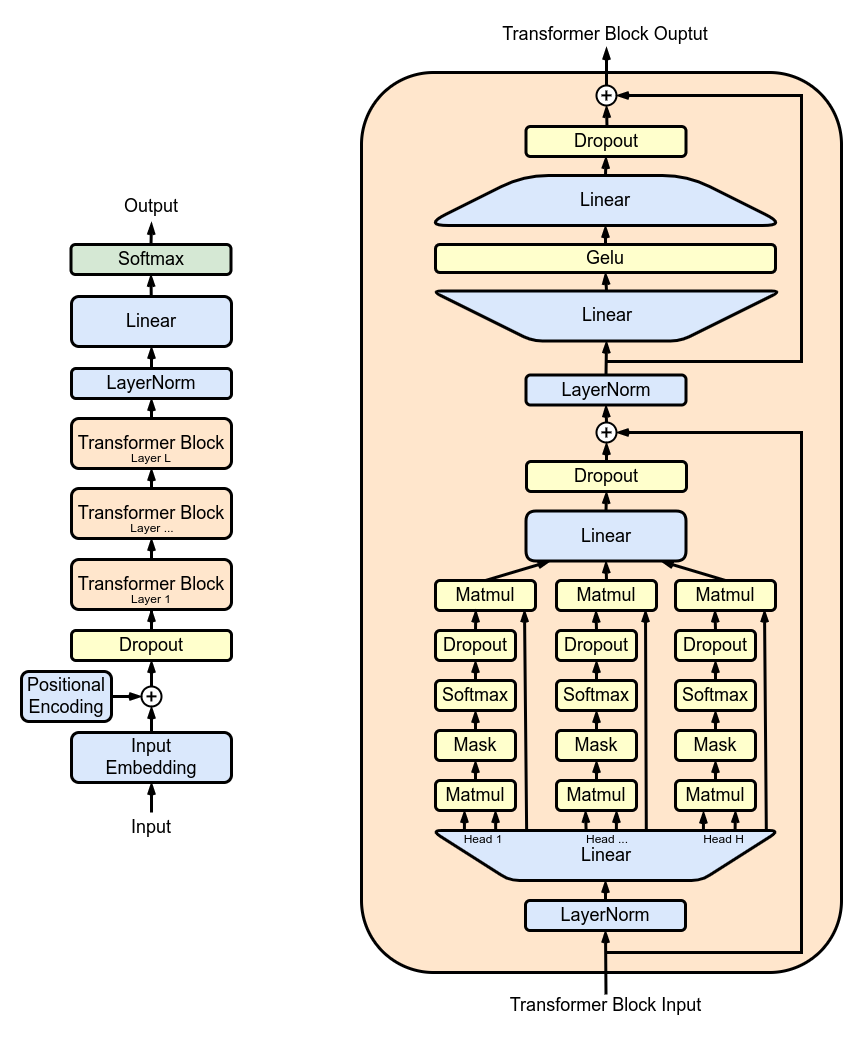
The diagram above, sourced from Wikipedia, illustrates the overall architecture of GPT and a transformer block. Let’s simplify our understanding of GPT. GPT is essentially a stack of transformer blocks. Since each block has the same architecture, we’ll focus on a single transformer block. A transformer block consists of three parts: a dense layer projection, self-attention, and a feed-forward network (two dense layers).
For simplicity, we’ll overlook some less important details related to computation and I/O, such as LayerNorm, Mask, Dropout, and residual connection. Instead, we’ll focus on matrix multiplications in our analysis. If you want a deeper understanding of the GPT architecture or the self-attention mechanism, I recommend reading the papers and blog posts listed at the end of this article.
GPT models come in different sizes, ranging from 125 million parameters to 175 billion parameters. Here’s a table outlining the hyperparameters of various GPT model sizes.
| Model | Layers (L) |
Heads (n) |
Attention Dim (d) |
Hidden Dim (h=n*d) |
|---|---|---|---|---|
| 125M | 12 | 12 | 64 | 768 |
| 350M | 24 | 16 | 64 | 1024 |
| 1.3B | 24 | 32 | 64 | 2048 |
| 6.7B | 32 | 32 | 128 | 4096 |
| 13B | 40 | 40 | 128 | 5120 |
| 30B | 48 | 56 | 128 | 7168 |
| 66B | 64 | 72 | 128 | 9216 |
| 175B | 96 | 96 | 128 | 12288 |
When using GPT to generate text, users provide a “prompt” to the model. The model processes the prompt, generating the first output token and two tensors known as “KV Cache.” We refer to this as the “Initial Stage.” Then, the model takes the previous output token and the KV cache as input, producing the next output token and an updated version of the KV cache. We refer to this as an “Auto-Regression” step. Auto-regression steps are repeated until the model generates the complete output.
Steps, FLOP, I/O
To enhance our understanding of a transformer block, I have created a table that lists the computation steps in a sequential manner. This allows us to read it from top to bottom, similar to executing a program.
The table provides not only the definition and output shape but also the number of FLOPs (floating point operations, i.e., the computation amount) and the number of I/O bytes (data transfer from GPU memory to GPU registers) for each step. When multiplying an NxM matrix with an MxP matrix to produce an NxP matrix, the FLOP count is N*M*P, and the I/O count is N*M + M*P + N*P. Additionally, we define the “Arithmetic Intensity” as FLOP : I/O.

Now, let’s closely examine this table together and discover some interesting insights:
- Parameters:
- Self-attention has
3h^2parameters, while the FFN (combined with the output projection) has9h^2parameters. - Self-attention accounts for only 1/4 of the total model parameters.
- Self-attention has
- Memory usage:
- The memory used by
Softmax(QK^T)isn*s^2. This is one of the reasons why longer context lengths pose challenges. For example, the 6.7B model with 32 heads requires16 GBof memory to store this temporary value for a 16k token input (32 * 16384^2 * sizeof(float16)). - In comparison,
Softmax(QK^T)V, as well asQ, K, V, and other hidden states, only usesn*d*smemory. In the previous example, it amounts to128 MB(4096 * 16384 * sizeof(float16)). K, Vneeds to be stored for subsequent auto-regression. In the previous example, the KV cache occupies256 MBper layer (128 * 2), and for the 6.7B model with 32 layers, the total KV cache takes up8 GB.
- The memory used by
- Time complexity:
- Transformers are known to have a quadratic relationship with sequence length, as demonstrated in the rows representing matrix multiplication for
Q, K, V. - More precisely, considering the dense layers, the overall time complexity is
O(s^2h + sh^2)for the initial stage andO(sh + h^2)for auto-regression. - Given that
h(> 4096) is usually much larger thans(< 2048), it is safe to say that the quadratic term of the embedding dimensionhis more significant than the sequence length.
- Transformers are known to have a quadratic relationship with sequence length, as demonstrated in the rows representing matrix multiplication for
- Matrix multiplications:
- A transformer block involves two types of matrix multiplications.
- The first type is the dense layer:
- A dense layer transforms an input vector to another vector using a vector-matrix multiplication.
- For higher-dimensional inputs, the vector-matrix multiplication is broadcasted to all dimensions except for the last one. For example, when applying a dense layer of shape
(h, h)to a tensor of shape(b, s, h), the tensor is reshaped to(b*s, h)before the matrix multiplication and then reshaped back to(b, s, h)afterward. - With a dense layer of shape
(h, h)and a batched input of shape(b, h), the compute intensity isO(1 / (1+1/b)). Increasing the batch size improves efficiency for dense layers.
- The second type is self-attention:
- As the name suggests, self-attention computes relationships among input tokens.
- For batched inputs, both
QandKhave a shape of(b, n, s, d). The operationQK^Trepresents a batched matrix multiplication. For thei-th entry of the batch and thej-th attention head,out[i, j] := matmul(Q[i, j, :, :], K[i, j, :, :].T). Asbincreases, both compute and I/O requirements increase, making arithmetic intensity unchanged.
- Batching for the initial stage:
- Dense layer:
- Due to the sequence length dimension, the input is already batched, even if the batch size is 1.
- We can consider it well-batched since the sequence length is usually long.
- Therefore, batching doesn’t significantly benefit the dense layer in the initial stage.
- Self-attention:
- As mentioned earlier, batching doesn’t increase the arithmetic intensity of self-attention. Thus, batching doesn’t help self-attention in the initial stage. (Not exactly… We’ll see in the next section.)
- Dense layer:
- Batching for auto-regression stages:
- Dense layer:
- Inputs to the dense layer in the auto-regression stage have the shape
(b, 1, h). - This is where batching brings substantial efficiency gains.
- Inputs to the dense layer in the auto-regression stage have the shape
- Self-attention:
- Unfortunately, batching doesn’t offer much improvement here. (Not exactly… We’ll see in the next section.)
- Dense layer:
- Batching end-to-end:
- Dense and self-attention:
- Batching helps dense layers but not self-attention.
- Dense layers accounts for 3/4 of the model parameters, indicating that it takes longer to execute than self-attention.
- Consequently, batching significantly benefits the entire model.
- Initial stage and auto-regression:
- The initial stage is already well-batched, and auto-regression benefits greatly from batching.
- Auto-regression steps are usually long, such as generating 100 or even 1000 tokens. Hence, auto-regression takes much longer than the initial stage.
- Therefore, batching significantly improves end-to-end text generation efficiency.
- Dense and self-attention:
Microbenchmarks
I decided to do some microbenchmarks to verify my understanding of the batching effects in the dense layer and self attention, as well as in the initial stage and the auto-regression.
The benchmark code is roughly like this:
def bench_dense(n, d, b, s):
  h = n * d
  X = torch.rand((b, s, h), dtype=torch.bfloat16, device="cuda")
  W = torch.rand((h, h), dtype=torch.bfloat16, device="cuda")
  def run():
    torch.matmul(X, W)
    torch.cuda.synchronize()
  latency = benchmark(run)

def bench_qk_init(n, d, b, s):
  Q = torch.rand((b, n, s, d), dtype=torch.bfloat16, device="cuda")
  K = torch.rand((b, n, s, d), dtype=torch.bfloat16, device="cuda")
  def run():
    torch.bmm(Q.view(b*n, s, d), K.view(b*n, s, d).transpose(1, 2))
    torch.cuda.synchronize()
  latency = benchmark(run)

def bench_qk_ar(n, d, b, s):
  Q = torch.rand((b, n, 1, d), dtype=torch.bfloat16, device="cuda")
  K = torch.rand((b, n, s, d), dtype=torch.bfloat16, device="cuda")
  def run():
    torch.bmm(Q.view(b*n, 1, d), K.view(b*n, s, d).transpose(1, 2))
    torch.cuda.synchronize()
  latency = benchmark(run)
I ran these benchmarks on NVIDIA A100 with PyTorch 2.0. The space of benchmark parameters is:
h = [768, 1024, 2048, 4096, 5120, 7168, 9216, 12288]
s = [1, 10, 20, 50, 100, 200, 500, 1000, 2000, 5000]
b = [1, 2, 3, 4, 5, 6, 7, 8,
     10, 12, 14, 16, 20, 24, 28, 32,
     40, 48, 56, 64, 80, 96, 112, 128]
Batching Overall

The figure above illustrates how batch size affects the throughput of the dense layer and self-attention in both the initial stage and auto-regression. Surprisingly, all four lines show significant improvements with batching.
The reason behind the benefit of batching for dense_init seems to be that the sequence length is small (50). The A100 easily handles the matrix multiplication of size 4096 x 4096 x 4096, and a batch size of 50 falls short of utilizing all available compute units.
How about a longer sequence length?

The above figure demonstrates similar results but with a sequence length of 1000. I’m still amazed to see that both qk_init and qk_ar experience benefits from batching, especially when comparing batch sizes of 1 and 4. It is possible that performing a matrix multiplication of 1000x128x1000 is simply too easy, even when running 32*b instances of such matrix multiplication in parallel. Another explanation could be that the matmul kernel is suboptimal and fails to make full use of the available computing units.
On the other hand, dense_init no longer observes any throughput gains from batching since the sequence length is already long. As previously analyzed, dense_ar continues to batch perfectly.
Batching of Dense Layer
Let’s take a closer look at dense layers.

The figure above shows throughput versus total FLOPs for various sizes of dense layers. This figure uses FLOPs as the x-axis, which is similar to b*s since FLOPs are O(bsh^2). Using FLOPs as the x-axis allows us to distinguish between different model sizes on the same plot.
The figure shows that no matter how big the model is, when the sequence length is not big, dense layers in the initial stage can benefit from batching to varying degrees before reaching the peak throughput.

The figure above shows the same plot for the auto-regression stage. Since the sequence length is always 1 for dense layers in the auto-regression stage, the batching effect has no (practical) upper limit.

What’s even better is that batching dense layers in the auto-regression stage doesn’t significantly affect latency, as shown in the figure above. Running with a batch size of 128 is almost as low-latency as running without batching. This is truly a free lunch!
Batching of Self Attention
Now, let’s examine self-attention.

During the initial stage, when the sequence length is shorter (s<=100), there is a significant impact on batching, but batching has minimal effect on longer sequences (s>=500).

The auto-regression stage follows a similar pattern because self-attention in both stages has the same FLOP:I/O ratio. Note that as auto-regression progresses, the sequence length increases, reducing the batching effect.

- The latency of self-attention is at the same magnitude as the latency of a dense layer.
- Unlike a dense layer, self-attention’s latency increases with batch size.
- The latency is approximately linear with respect to the batch size. This is because self-attention is essentially batched matrix multiplication. With a fixed FLOP:I/O ratio, batching implies more work without gaining speed on individual tasks.
- Once again, as auto-regression continues, the sequence length increases, requiring more time to process each step.
Roofline Model

The figure above depicts the data points of all benchmark combinations, following the concept of a Roofline Model. The four colors represent different stages and layers. Each color includes a lighter version, demonstrating the data points of the 6.7B model as an example. Additionally, the figure displays the theoretical memory bandwidth and FLOP/s from NVIDIA A100 specs.
There are two notable aspects of this figure. First, the data points group into clusters and sub-clusters. Second, the data points closely align with the theoretical roofline.
To observe the impact of batching, let’s examine a specific case (h=4096, s=100):

From these two figures, we can gather the following insights:
- Arithmetic intensity follows the order:
dense_init > qk_init > dense_ar > qk_ar. - Achieved FLOP/s follows the order:
dense_init > qk_init > dense_ar > qk_ar. - The dense layer in the initial stage is limited by the peak computing performance of the GPU. When the sequence length is short and the model is small, batching can provide a slight improvement. Otherwise, the only solution for enhancement is to invest in a more powerful GPU.
- Data points of the dense layer in the auto-regression stage of the same model size form a line. This line has the same slope as the GPU’s memory bandwidth. Consequently, the dense layer in the auto-regression stage is bounded by memory bandwidth. Increasing the batch size increases the achieved FLOP/s under the memory bandwidth constraint by elevating the arithmetic intensity.
- Batching does not change the arithmetic intensity of self-attention. However, in cases with a short sequence length, batching increases the achieved FLOP/s of self-attention through parallel processing. The fact that the achieved FLOP/s increases without changing the arithmetic intensity implies that the kernel implementation of self-attention may be suboptimal, not utilizing all compute units.
Text Generation End-to-end Benchmark
In the previous section, we conducted microbenchmarks for the dense layer and self-attention. Now, let’s examine how batching affects text generation through an end-to-end benchmark. For this benchmark, I used the 6.7B model with an input token length of 200 and an output token length of 500.

The figure above illustrates the latency of the initial stage and each auto-regression step at different batch sizes. Several interesting observations can be made from this figure:
- The latency of the auto-regression step is comparable to that of the initial stage. Considering the generation of hundreds of new tokens, the total latency is primarily influenced by auto-regression.
- The initial stage exhibits a slight batching effect, with latencies of 24ms for
b=1and 119ms forb=8. - The auto-regression steps demonstrate a significant batching effect. The last token (which is the slowest) takes 14ms for
b=1and 24ms forb=8.
Based on these observations, we can make an educated guess that batching can significantly increase throughput while only slightly impacting latency.

| b | Latency Penality | Relative Throughput |
|---|---|---|
| 1 | 0 | 1x |
| 2 | + 3% | 1.93x |
| 3 | + 8% | 2.75x |
| 4 | +14% | 3.48x |
| 5 | +21% | 4.11x |
| 6 | +28% | 4.67x |
| 7 | +34% | 5.18x |
| 8 | +41% | 5.65x |
| 10 | +53% | 6.49x |
| 12 | +67% | 7.16x |
| 14 | +81% | 7.70x |
| 16 | +94% | 8.23x |
The figure and table above confirm this guess:
- At a batch size of 2, latency remains almost the same, but the throughput nearly doubles.
- At a batch size of 4, latency increases by 14%, while the throughput improves by a factor of 3.5.
- The latency is roughly linear with batch size.
- Here’s how we can understand it.
- The latency contains one initial stage and 500 auto-regression steps. As mentioned earlier, auto-regression predominantly affects latency. Therefore, we focus on the auto-regression stage.
- Referring back to the figures in the microbenchmark section, we observe that the latency of self-attention scales linearly with batch size, whereas the latency of the dense layer remains nearly constant regardless of batch size.
- Despite dense layers takes a few more times to run than self-attention, the latter still contributes significantly to the overall latency of the entire layer. Hence, the linear relationship between latency and batch size extends to the entire layer.
- Additionally, as batch size increases, the rate of throughput improvement diminishes.
- We can use a simple analytical model to understand this diminishing return.
- Let’s assume the latency of batch size
bis represented asc0 + c1 * b, wherec0andc1are positive constants. - The throughput of batch size
bcan be calculated asb / (c0 + c1 * b). - The slope of the throughput, given by
c0 / (c0 + c1 * b)^2, is always positive (indicating an increase in throughput with larger batch sizes) but decreases (implying diminishing returns).
- The difference in latency between batch sizes 1 and 2 is small compared to the gaps between larger batches.
- This is because batch size 1 doesn’t fully utilize all available compute units. Therefore, when running with a batch size of 2, we experience some additional efficiency without incurring significant latency penalties.
Improve LLM Serving
Having gained expertise in LLM performance, let’s figure out how to enhance LLM serving based on our findings.
Fuse Self Attention
As we previously analyzed, QK^T generates a temporary output of shape (b, n, s, s), while we only require the final result of Softmax(QK^T)V, which has the shape (b, n, s, d). Since d=128 is relatively small, we can fuse the multiplication of these three matrices into a single cuda kernel, directly producing (QK^T)V.
However, there’s an obstacle: Softmax. The typical softmax implementation requires reading all numbers in the last dimension of QK^T. This poses a problem since we can only compute a block of QK^T while fusing the multiplication with V. To overcome this limitation, we need a clever way to compute softmax, ensuring it remains associative. Thankfully, some smart people have already discovered the approach known as Online Softmax. We can try implementing this technique and work out the necessary details.
Congratulations! We’ve essentially reinvented the FlashAttention [NeurIPS’22] paper. Additionally, I recommend checking out this awesome notes on FlashAttention.
Batch Across Requests
Another significant opportunity lies in batching requests together, resulting in a substantial increase in throughput while incurring minimal latency penalties, as we discussed earlier. LLM services like OpenAI ChatGPT and HuggingFace Hosted Inference can greatly benefit from batching.
During our analysis, we made the simplifying assumption that all requests have the same length. However, in reality, requests varies in length. While padding all requests to the same length is an option, it also increases computation. Fortunately, we can devise a more efficient solution by revisiting our previous findings:
- Dense layers exhibit a strong batching effect, with latency remaining nearly constant regardless of batch size during auto-regression.
- Dense layers do not consider the concept of a “sequence”; instead, a “sequence” is treated as another batching dimension.
- Self-attention, by definition, must compute against the same sequence and cannot be batched.
- Nonetheless, dense layers still take longer to execute than self-attention, so there is still much to gain by batching only dense layers.
Based on these observations, we can propose a remarkably simple approach to batch multiple sequences together:
- Given inputs of shapes
[(s1, h), (s2, h), ...], we stack them into a large matrix of shape(sum(si), h). - Apply the dense layer to this stacked matrix.
- Split the result of the dense layer back into
[(s1, h), (s2, h), ...]. - Perform self-attention for each sequence individually.
Congratulations! We’ve essentially reinvented the Orca [OSDI’22] paper.
Summary
- We have condensed computation steps of a transformer block, FLOPs, I/O, and arithmetic intensity into a table.
- We have analyzed the effects of batching on dense layers and self-attention, considering both the initial stage and auto-regression.
- To validate our analysis, we have conducted microbenchmarks and explained the results using the roofline model.
- We have performed an end-to-end benchmark of text generation, demonstrating that batching significantly improves throughput with only a minor increase in latency.
- We have (re-)discovered techniques to enhance LLM serving by combining self-attention and batching across requests.
I would like to thank Zihao Ye and Zhipeng Jia for their inspiration and insightful discussions.
If you want to reproduce the microbenchmarks, you can download this notebook. If you want to inspect the microbenchmark data, you can download this CSV.
More to Read
- Understanding Self-Attention, Transformer, GPT
- Papers
- Blog posts
- Code
- OPT implementation from HuggingFace Transformers library in PyTorch.
- Performance Improvement
- Performance Analysis